Moving Averages
To clarify the long term trend, a technique called smoothing can be used where groups of values are averaged.
The graph of moving mean or moving medians is "flatter" than the time series graph with its peaks and troughs.
The average can be either a moving mean or a moving median. In this process the mean or median of groups of values are taken. If a group of 4 values is used it is said to be of order 4.
Moving median − odd number of cycles
The following table shows the sales in millions ($) year period of a company.
The moving medians (order 3) are calculated by:
Finding the median of values 1 to 3 and placing this median next to the second value,
Finding the median of values 2 to 4 and placing this median next to the third value.
etc., etc.
|
Year
|
Sales($millions)
|
Moving median |
|
1990
|
37
|
|
|
1991
|
45
|
39
|
|
1992
|
39
|
45
|
|
1993
|
48
|
47
|
|
1994
|
47
|
48
|
|
1995
|
57
|
52
|
|
1996
|
52
|
52
|
|
1997
|
49
|
52
|
|
1998
|
56
|
56
|
|
1999
|
59
|
59
|
|
2000
|
62
|
Note there will not be a moving median for the first and last values
The graph of the original data and the moving medians is shown below:
The long term trend can now be seen more clearly.
There are three possibilities:
- No long term trend − the moving average line would be flat.
- An additive trend where the moving average line slopes up or down.
- A multiplicative trend where the moving average line is curved. e.g. Population growth or inflation.
In the case above there would appear to be a increasing or additive trend.
Moving mean − even number of cycles
The data below shows sales of a company for two years.
As the data is obviously seasonal, arranged in 4 quarters each year, then the data should be smoothed using groups of four.
The moving means are worked out in a similar manner to the moving medians.
i.e. 31.75 is the mean of 27, 45, 34 and 21.
The problem now is where to put the moving means!
To get around this problem extra rows are put in between each value. To enable a moving mean to be placed next to the values the centred mean , which is the average of the moving means, are placed in another column.
i.e. 32.375 is the average of 32 and 32.75
| Year | Quarter |
Sales ($ millions)
|
Moving mean
|
centred means
|
| 1999 |
1
|
27
|
||
|
2
|
45
|
|||
| 31.75 | ||||
|
3
|
34
|
31.875 | ||
| 32 | ||||
|
4
|
21
|
32.25 | ||
| 32.5 | ||||
| 2000 |
1
|
28
|
32.25 | |
| 32 | ||||
|
2
|
47
|
32.375 | ||
| 32.75 | ||||
|
3
|
32
|
|||
|
4
|
24
|
Using a Spreadsheet for Smoothing
Spreadsheets are ideal for graphing time series and carrying out the smoothing process.
The example below shows the smoothing (moving mean − order 5) and graphing of time series data of company sales figures.
From the smoothed graph the upward trend of increasing sales can be clearly seen.
Seasonally Adjusted Data
When the data has been smoothed and trends analysed, each value can be looked at for seasonal effects. This is to see if the values are significantly different from what might be expected and to help make predictions.
|
Individual seasonal effect = value − moving average
|
To show how this works, the bicycle company's figures will be used. As the data is for days of the week a moving mean of 7 is chosen.
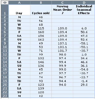 |
Seasonal effect e.g. For Saturday the seasonal effect is the average of 47.0 and 46.6 which is 46.8 To seasonally adjust a particular value:
e.g. For the second Saturday:
|
Interpretation of Adjusted Values
A seasonally adjusted value is more than expected if it is above the corresponding moving mean value.
e.g. For the second Saturday, the value of 99.2 is a little below what could have been expected (99.4)
Predicting and Forecasting Future Values
To predict values in the future from existing time series data requires the calculation:
|
Predicted value = estimated moving mean + seasonal effect
|
The estimated moving mean in the formula above can be worked out in several ways.
1. Use the table above to work out by how much the moving mean is changing each day.
To predict the value of the fourth Saturday, assume that the moving mean will continue to decrease by about 1 each day as in the table.
Predicted value = 94.0 + 8 x (-1) + 46.8 = 132.8
2. Draw a graph of the moving means and insert a trend line. Use the gradient of the trend line to predict future values:
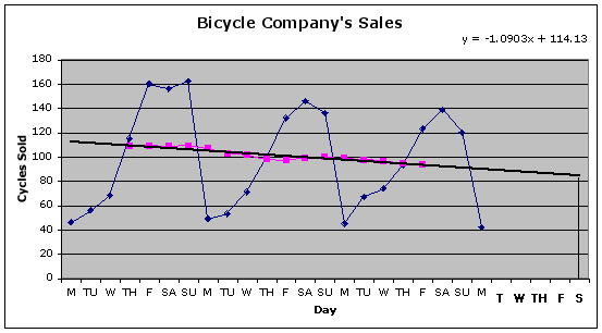
The trend line has been extended to go to the next Saturday. Using the graph the number of cycles sold on the final Saturday can be estimated:
Predicted value = Estimated moving mean + seasonal effect for Saturday = 84 + 46.8 = 130.8
OR
The equation of the trend line can be worked out from the graph or calculated by the spreadsheet, as above. This equation is used with an x-value equal to the number of time periods. In the graph above, there are 27 days therefore x = 27.
y = -1.0903 x 27 + 114.13 = 84.7
Add on the seasonal effect for Saturday, predicted value = 84.7 + 46.8 = 131.5