1. The time series in the following table gives numbers of registered unemployed in a city on 31 March, 31 July and 30 November over the last five years. The means of successive sets of three terms in the time series and individual four-month seasonal effects are included, with one value missing in each of the three columns.
|
Year
|
Time
|
Number
|
Mean of three
|
Individual Seasonal Effects
|
| 1992 | 31 July |
3210
|
||
| 30 November |
2843
|
2940
|
-97
|
|
| 1993 | 31 March |
2767
|
2877
|
-110
|
| 31 July |
3021
|
2800
|
221
|
|
| 30 November |
2612
|
2726
|
-114
|
|
| 1994 | 31 March |
2545
|
2684
|
-139
|
| 31 July |
2895
|
2611
|
284
|
|
| 30 November |
2393
|
2534
|
-141
|
|
| 1995 | 31 March |
2314
|
-
|
-
|
| 31 July |
2631
|
2371
|
260
|
|
| 30 November |
2168
|
2292
|
-124
|
|
| 1996 | 31 March |
2077
|
2213
|
-136
|
| 31 July |
2394
|
a. Explain the purpose of smoothing the time series.
b. Calculate the missing mean of three terms and the missing seasonal effect for 31 March 1995.
c. Use the individual seasonal effects to obtain estimates for the seasonal effects for 31 March, 31 July and 30 November.
d. Seasonally adjust the number unemployed on 31 July 1996 using the result in 1.c and comment on the claim by the local mayor that unemployment is rising in the city.
e. Assuming that the trend continues to change by 79 registered unemployed at the end of each successive four-monnth interval, use the estimates of the seasonal effects from 1.c. to forecast unemployment levels on 30 November 1996, 31 March 1997 and 31 July 1997.
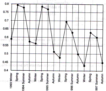
2. a. A particular motel's occupancy rate for each of the four seasons over the last four years is shown in the time series plot below. State any two components of the time series for the motel's occupancy rate that are visible in this plot.
|
Motel's Occupancy Rate (Winter 1993 − Autumn 1997)
|
 |
b. The time series for the motel's occupancy rate is shown in the table below. Also included in the table are:
Moving mean − the mean of four successive terms in the time series for the motel's occupancy rate.
Centred Moving Mean - the mean of two successive moving means.
Individual Seasonal Effects − the difference between the occupancy rate and the centred moving mean.
One value (shown by an asterisk * in each case) is missing from each of the last three columns.
|
Year
|
Season
|
Occupancy Rate
|
Moving Mean
|
Centred Moving Mean
|
Individual Seasonal Effects
|
| 1993 |
Winter
|
0.590 |
|||
|
Spring
|
0.793
|
||||
|
0.6835
|
|||||
| 1994 |
Summer
|
0.778
|
0.6800
|
0.0980
|
|
|
0.6765
|
|||||
|
Autumn
|
0.573
|
0.6755
|
- 0.1025
|
||
|
0.6745
|
|||||
|
Winter
|
0.562
|
0.6733
|
- 0.1113
|
||
|
*
|
|||||
|
Spring
|
0.785
|
0.6644
|
0.1206
|
||
|
0.6568
|
|||||
| 1995 |
Summer
|
0.768
|
0.6460
|
0.1220
|
|
|
0.6353
|
|||||
|
Autumn
|
0.512
|
0.6239
|
- 0.1119
|
||
|
0.6125
|
|||||
|
Winter
|
0.476
|
0.5950
|
-0.1190
|
||
|
0.5775
|
|||||
|
Spring
|
0.694
|
*
|
0.1183
|
||
|
0.5740
|
|||||
| 1996 |
Summer
|
0.628
|
0.5681
|
0.0599
|
|
|
0.5623
|
|||||
|
Autumn
|
0.498
|
0.5540
|
-0.0560
|
||
|
0.5458
|
|||||
|
Winter
|
0.429
|
0.5424
|
-0.1134
|
||
|
0.5390
|
|||||
|
Spring
|
0.628
|
0.5325
|
*
|
||
|
0.5260
|
|||||
| 1997 |
Summer
|
0.601
|
|||
|
Autumn
|
0.446
|
(i) Calculate the missing values (shown by an asterisk *) the moving mean for Winter-Spring 1994; the centred mean for Spring 1995; and the individual seasonal effect for Spring 1996.
(ii) Use the individual Summer seasonal effects to estimate the seasonal effect for Summer.
(iii) Seasonally adjust the occupancy rate for Summer 1996. Show your working.
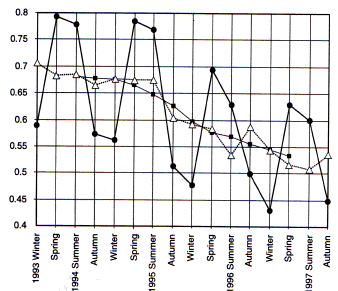
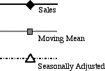
c. The occupancy rates, the centred moving means and the seasonally adjusted occupancy rates for the motel are shown in the plot below.
 |
 |
(i) What do the centred moving means show us about the motel's occupancy rates over this period of time?
(ii) Was the occupancy rate for Autumn 1996 better or worse than expected? Justify your answer using the information shown in this plot.
(iii) Assuming that the centred moving means for the motel's occupancy rate continue to change by 0.01 for each season, use the estimate of the seasonal effect for Summer in c. (ii) to forecast the motel's occupancy rate for Summer 1998.
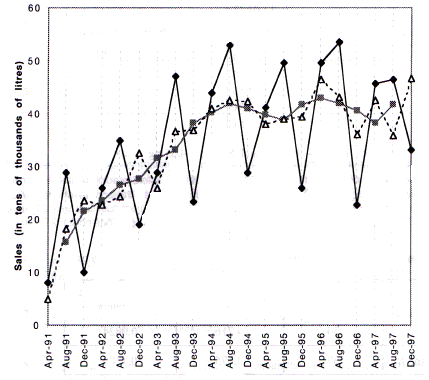
3. A chemical company produces a herbicide (weed killer) for the agricultural and residential market. The company's total herbicide sales in tens of thousands of litres for four-month periods over the last 7 years (the raw sales data) are shown in the time series plot below. Also shown in the plot are moving means and the seasonally adjusted data.
|
Herbicide Sales (1991 − 1997)
|
 |
|
Period Ending
|
(i) Randomness is one of the components of general time series analysis that is visible in the raw sales data in this plot. State two other components that are visible in this plot.
(ii) Describe a feature (visible in this plot) of one of the components that you have given in part (i).
(iii) How many seasonal effects need to be estimated in order to determine the seasonally adjusted data?
(iv) Was the sale of herbicide for August 1997 more than expected? Justify your answer using the information shown in this plot.
