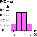
 The binomial distribution is a common type of probability distribution which obeys certain conditions. In an experiment:
- There are only two possible outcomes (usually called successes or failures)
- There are a fixed number of trials (n)
- Each trial must be independent of the other trials
- The probability of success (π) is fixed at each trial
n and π are called parameters of the distribution.
Example of a Binomial Distribution
An example of an experiment which would result in a binomial distribution is the tossing of a coin 3 times and counting the number of heads.
Check that it is a binomial distribution:
| There are only two possible outcomes. |
Success: getting a head |
| There are a fixed number of trials. | The coin is tossed three times (n = 3) |
| Each trial must be independent. | The first toss does not effect the second, etc. |
| The probability of success is fixed. | Each time the probability of a head is 0.5 (π = 0.5) |
For our experiment the possible outcomes are given below.
The probability of each outcome will be 0.5 x 0.5 x 0.5 = 0.125.
|
Number of heads (x)
|
0
|
1
|
2
|
3
|
 |
|
Outcomes
|
TTT
|
HTT
THT TTH |
HHT
HTH TTH |
HHH
|
|
|
P( X = x)
|
0.125
|
0.375
|
0.375
|
0.125
|
Binomial Probability from Formula
The formula for binomial probability is:
|
x is the number of successes
|
Example
What is the probability that two heads will result when three coins are tossed?
| n = 3 (number of trials) x = 2(number of successes) π = 0.5 (probability of a success) |
P(X = 2) = 3 x 0.52 x 0.51 = 0.375 (which is same as the value in the probability distribution above).
Binomial Probability from Tables
Rather than use the formula for finding binomial probabilities, tables are available to look these up.
A table of the Binomial Distribution for values of n from 4 to 10 and values of π from 0.05 to 0.5 are given with the Bursary examination. The example above cannot be done using tables as n = 3
Use the tables to find the probability that two heads result when FOUR coins are tossed
The part of the table for for n = 4, x = 2 and π = 0.5 is shown below:
| n |
x
|
0.05
|
0.1
|
0.15
|
1/6
|
0.2
|
0.25
|
0.3
|
1/3
|
0.35
|
0.4
|
0.45
|
0.5
|
| 4 |
0
|
0.8145
|
0.6561
|
0.522
|
0.4813
|
0.4096
|
0.3164
|
0.2401
|
0.1975
|
1785
|
0.1296
|
0.0915
|
0.0625
|
|
1
|
0.1715
|
0.2916
|
0.3685
|
0.3858
|
0.4096
|
0.4219
|
0.4116
|
0.3951
|
0.845
|
0.3456
|
0.2995
|
0.25
|
|
|
2
|
0.0135
|
0.0486
|
0.0975
|
0.1157
|
0.1536
|
0.2109
|
0.2646
|
0.2963
|
0.3105
|
0.3456
|
0.3675
|
0.375
|
|
|
3
|
0.0005
|
0.0036
|
0.0115
|
0.0154
|
0.0256
|
0.0469
|
0.0756
|
0.0988
|
0.1115
|
0.1536
|
0.2005
|
0.25
|
|
|
4
|
0.0001
|
0.0005
|
0.0008
|
0.0016
|
0.0039
|
0.0081
|
0.0123
|
0.015
|
0.0256
|
0.041
|
0.0625
|
Interestingly, the probability of getting two heads when four coins are tossed is the same as when three coins are tossed!
If the above question asked for the probability that there are two or fewer heads i.e. P(X < 3) then the probabilities for x = 0, 1 and 2 would need to be added together.
P(X < 3) = 0.375 + 0.25 + 0. 0625 = 0.6875
Sometimes if the probability of a success is greater than 0.5 the probability of obtaining the corresponding number of failures should be found using 1 − π which will be in the tables.
Example
The probability that a key works in a lock is 0.9. If the key is used 10 times find the probability that the key works 8 times.
Let x be the number of times the key does not work. (Because π = 0.9 is too large for the tables.)
Therefore we are looking for 2 failures so x = 2 with π = 0.1, n = 10
From tables P(X = 2) = 0.1937
Mean and Variance of the Binomial Distribution
When three coins are tossed, X is the number of heads.
|
Number of heads (x)
|
0
|
1
|
2
|
3
|
|
P( X = x)
|
0.125
|
0.375
|
0.375
|
0.125
|
E(X) = μ = 0 x 0.125 + 1 x 0.375 + 2 x 0.375 + 3 x 0.125 = 1.5
VAR(X) = E(X2) − [E(X)]2 = 02 x 0.125 + 12 x 0.375 + 22 x 0.375 + 32 x 0.125 − 1.52 = 0.75
SD(X) = √VAR(X) = √0.75 = 0.866 (to 3 sig.figs.)
There are formulae for working the mean, variance and standard deviation of a binomial distribution.
| Mean (expected value) | μ = np |
| Variance |
σ2 = npq |
| Standard deviation | σ = √(npq) |
In the example above:
E(X) = μ = np = 3 x 0.5 = 1.5
VAR(X) = npq = 3 x 0.5 x 0.5 = 0.75
SD(X) = √(npq) = √(3 x 0.5 x 0.5) = 0.866 (to 3 sig.figs.)