This topic covers mathematical modelling, which is a process where mathematical equations are found to fit or approximate real life situations and data. The two most common types of functions which occur in real life situations are exponential functions and power functions. The previous topic covered exponential modelling. Both processes involve the use of logarithms and you should be familiar with the rules of logarithms covered in Year 11.
The Power Function
The general form of an power function can be given as:
y = Ax n
Given a set of values (x , y) from an experiment or survey, the problems are:
- Do these values fit into the power function model?
- How are the values of A and n found?
To answer these questions, we manipulate y = Ax n using logarithms:
Take natural logs of both sides:
|
ln y
|
=
|
ln Ax n |
|
ln y
|
=
|
ln A + ln x n |
|
ln y
|
=
|
ln A + n ln x |
|
ln y
|
=
|
n ln x+ ln A |
This equation can be seen to fit the pattern of a straight line y = mx + c.
This means that from our original set of values (x, y) if we plot (ln x , ln y) we should get a straight line. If we do get a straight line this confirms that the power function y = Axn is a suitable model and we can proceed to find the values of A and n. The y- intercept of the line will be ln Aand the gradient of the line will be n.
Example
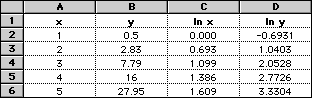
We wish to show that the values in the table below can be modelled using an power function:
|
x
|
1
|
2
|
3
|
4
|
5
|
|
y
|
0.50
|
2.83
|
7.79
|
16.00
|
27.95
|
We now take natural logs of each y value and each x value and sketch them on a graph to see if they form a straight line. This will be done on a spreadsheet. (Log -log graph paper could be used. Log-log graph paper has both axes with a logarithmic scale and both the x-value and the y-value is plotted straight onto graph − a straight line will result if the exponential model is suitable.)
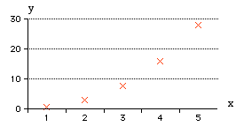
| The graph of x against y clearly looks like a power functionl. Seeming to pass through (0, 0) and be less steep than most exponential functions | The graph of ln y against ln x confirmsthis − it is a straight line. |
 |
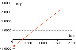 |
The values will be modelled by y = A x n
Remember ln y =n ln x + ln A
| To find the value of n | To find the value of A |
|
The value of n is the gradient of the straight line. Use any 2 values from the table:
n = 2.49 (to 2 d.p.)
|
The value of ln A is the y-intercept of the graph or can be found using the equation. ln y = n ln x + ln A ln 7.79 = 2.49 x ln 3 + ln A ln A = 2.0528 − 2.7355 ln A = -0.6827 A = 0.51 (to 2 d. p.) |
|
The values can be modelled by the power function y = 0.51x2.49
|
|
Use this simulation to be able to plot log graphs − ![]()
Predicting Values
In the problem above, now that the equation y = 0.51x2.49 has been found, other values can be calculated.
Example
Find the value of x if y = 50.
50 = 0.51x2.49
x2.49 = 98.04
Take natural logs of both sides.
ln x2.49 = ln 98.04
2.49 ln x = ln 98.04
ln x = ln 98.04 / 2.49
x = 6.3061 (to 5 sig. fig.)